Installing Zresidual and Other packages
Installing Z-residua from the source
Intalling and Loading R Packages used in this Demo
Code
# Vector of required packages
pkgs <- c(
  "survival","EnvStats","foreach", "statip", "VGAM", "plotrix", "actuar",
  "stringr", "Rlab", "dplyr", "rlang", "tidyr",
  "matrixStats", "timeDate", "katex", "gt","loo"
)

# Check for missing packages and install if needed
missing_pkgs <- pkgs[!pkgs %in% installed.packages()[, "Package"]]
if (length(missing_pkgs) > 0) {
  message("Installing missing packages: ", paste(missing_pkgs, collapse = ", "))
  install.packages(missing_pkgs, dependencies = TRUE)
} else {
  message("All required packages are already installed.")
}

# Load all packages
invisible(lapply(pkgs, library, character.only = TRUE))

options(mc.cores = parallel::detectCores())
Introduction
This vignette demonstrates how to use the Zresidual package to compute Z-residuals for diagnosing Logistic regression, based on the output from the brms package in R (Bürkner 2017) to reveal potential model misspecifications. The examples illustrate the practical use of these residuals for RPP (Feng, Li, and Sadeghpour 2020) diagnostics.
Definitions of Z-residuals for Logistic Regression
This section demonstrates the definitions of posterior predictive quantities including the posterior predictive PMF, survival function, and RPP for Logistic Regression.
Let y_i \in \{0, 1\}, where y_i = 1 indicates a success, and y_i = 0 indicates a failure for the i^th observations.
Using Bayesian estimation (e.g., via the brms package), we draw T samples from the posterior distribution. Let \theta^{(t)} denote the t^{th} posterior draw.
For a given observation y_i^\text{obs}, the posterior predictive PMF and survival functions are defined below.
\begin{equation}
p_i^{\text{post}, \text{logit}}(y_i^\text{obs}) = \frac{1}{T} \sum_{t=1}^T
\begin{cases}
{\pi^o_i}^{(t)} & \text{if } y_i^\text{obs} = 1, \\
1 - {\pi^o_i}^{(t)} & \text{if } y_i^\text{obs} = 0,\\
0 & \text{otherwise.}
\end{cases}
\end{equation}
\begin{equation}
S_i^{\text{post}, \text{logit}}(y_i^\text{obs}) = \frac{1}{T} \sum_{t=1}^T
\begin{cases}
1 & \text{if } y_i^\text{obs} < 0, \\
1-{\pi^o_i}^{(t)} & \text{if } 0 \le y_i^\text{obs} < 1, \\
0, & \text{if } y_i^\text{obs} \ge 1.
\end{cases}
\end{equation}
For any observed value y_i^\text{obs}, we define: \begin{equation}
\label{eq:post_rpp}\text{rpp}_i(y_i^\text{obs} | \theta^{(t)}) = S_i(y_i^\text{obs} | \theta^{(t)}) + U_i \times p_i(y_i^\text{obs} | \theta^{(t)})
\end{equation} where U_i \sim \text{Uniform}(0,1). Here, y_i^\text{obs} is the observed value, which can refer to either success or failure. Then, the Z-residual of the response variable is, \begin{equation}
\label{eq:z_residual}
z_i = -\Phi^{-1}(\text{rpp}_i(y_i^\text{obs}|\theta)) \sim N(0, 1)
\end{equation} where (^{-1}(.)) is the quantile function of standard normal distribution.
A Simulation Example
Model fitting with brms
To demonstrate how Zresidual works with hurdle models, we first simulate data from a HNB model. This simulated dataset allows us to evaluate how well the model and residual diagnostics perform when the true data-generating process is known.
Code
# Simulation parameters
n <- 100
beta0 <- -1
beta1 <- 6
beta2 <- 1

# Predictors
x1 <- runif(n, 0, 1)
x2 <- rbinom(n, size = 1, p = 0.5)

# Generating response variable
logit_p <- beta0 + beta1*x1 + beta2*x2
p <- exp(logit_p) / (1 + exp(logit_p))
y <- rbinom(n, 1, p)

# Random error variables
j <- 5 # number of random effect
sample_experiment <- replicate(j, rnorm(n, mean = 0, sd = 1), simplify = FALSE)
z <- data.frame(matrix(unlist(sample_experiment), ncol=j, byrow=FALSE))
z_names <- paste0("z", seq(1,j))
colnames(z) <- z_names

data_logit <- data.frame(x1, x2, z, y)

k <- j+2
predictors <- colnames(data_logit)[2:k]
logit_formula <- formula(paste("y ~ ", paste(predictors, collapse=" + ")))
This dataset includes a continuous predictor x1, binary variable x2, and five random error variables z1, z2, z3, z4, z5 and the outcome y is generated from a Bernoulli process. Note that the error variables are not included in generating the y outcome variable.
Now, we use the brms package to fit a logistic regression model to the simulated data.
The family = bernoulli() tells brms to use a logistic regression for binary response. We use default parameter setting on this example to fit the model.
Computing Z-residuals
In this example, we compute Z-residuals for the logistic regression using Zresidual.bernoulli(). The package take brms fit as an input for the Zresidual.bernoulli() function. If the model is Hurdle model, the type argument ("zero", "count" or "hurdle") specifies which component to use when calculating the residuals. By default, Z-residuals are computed using the Importance Sampling Cross-Validation (iscv) method based on randomized predictive p-values (RPP). Alternatively, users can choose the standard Posterior RPP method by setting method = "post".
Code
zres_logit_iscv <- Zresidual(fit_logit)
zres_logit_post <- Zresidual(fit_logit, method = "rpost")
What the function returns
The function Zresidual.bernoulli() (and other Z-residual computing functions) returns a matrix of Z-residuals, with additional attributes. The returned object is of class zresid, which includes metadata useful for diagnostic and plotting purposes.
Return Value
A numeric matrix of dimension n × nrep, where n is the number of observations in the data and nrep is the number of randomized replicates of Z-residuals (default is 1). Each column represents a set of Z-residuals computed from a RPP, using either posterior (post) or importance sampling cross-validation (iscv) log predictive distributions.
Matrix Attributes
The returned matrix includes the following attached attributes:
-
type: The component of the hurdle model the residuals correspond to. One of “zero”, “count”, or “hurdle”. For logistic, type is returned as “zero”.
-
zero_id: Indices of observations where the response value was 0. Useful for separating diagnostics by zero and non-zero parts.
-
log_pmf: A matrix of log predictive probabilities (log-PMF) per observation and posterior draw.
-
log_cdf: A matrix of log predictive CDF values used in computing the RPPs.
-
covariates: A data frame containing the covariates used in the model (excluding the response variable). This can be used for plotting or conditional diagnostics.
-
fitted.value: The posterior mean predicted value for each observation depending on the type.
Visualizing Z-residuals
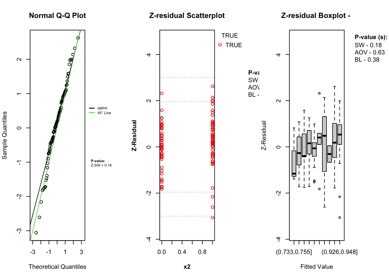
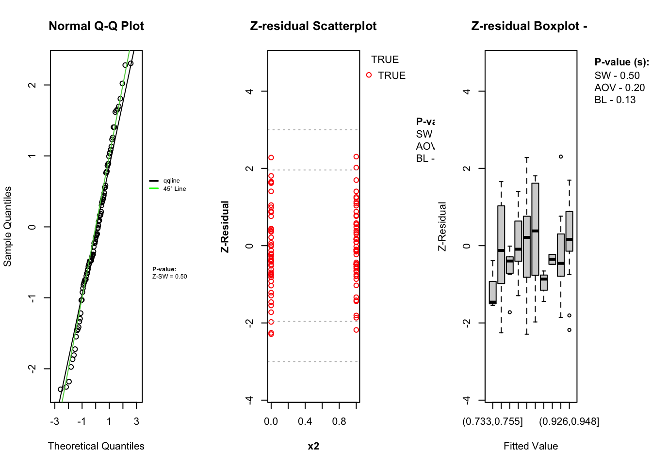
The Zresidual package includes built-in plotting functions (QQ Plot, Scatter Plot, Boxplot) to help diagnose model fit using Z-residuals. These functions are designed to work directly with objects of class zresid returned by functions like Zresidual.bernoulli(). These plots help assess:
-
Whether residuals are approximately standard normal (via QQ plots),
-
Whether there are patterns in residuals across fitted values (which may suggest model misspecification),
-
Whether residuals differ across covariates (optional extensions).
The diagnostic evaluations for the model—comprising scatter plots, Q-Q plots, and boxplots of Z-residuals—demonstrate that the model adequately captures the data structure. The Z-residuals are evenly scattered around zero and mostly fall within the range of -3 to 3, indicating no visible model misfit. The “count” represent success while “zero” represent failure. Complementary statistical tests, including the SW test for normality, ANOVA for mean equality, and BL test for variance homogeneity, all return p-values above the 0.05 threshold. This suggests that the residuals follow a normal distribution and exhibit equal means and variances across fitted value intervals. The Q-Q plots further support normality through close alignment with the 45-degree reference line, while the boxplots confirm consistent residual means across partitions. Collectively, these diagnostics validate that the model satisfies key distributional assumptions and that the proposed Z-residual methods are effective in detecting model adequacy.
The plotting functions in the Zresidual package are designed to be flexible and lightweight, allowing users to quickly visualize residual patterns. These functions support all customizable arguments in base R functions such as axes, labels etc. by making them adaptable to a wide range of diagnostic workflows. The plot.zresid() function offers flexible diagnostic plotting for Z-residuals, supporting various x-axes such as index, fitted values, and covariates. Both plot.zresid() and qqnorm.zresid() automatically highlights outlier residuals that fall outside the typical (or user specified) range making it easier to identify problematic observations.
Statistical Tests
In addition to visual diagnostics, the package offers formal statistical tests to quantify deviations from normality or homogeneity of variance in Z-residuals by taking an zresid class object as an input.
Shapiro-Wilk Test for Normality (SW)
Analysis of Variance (ANOVA)
Bartlett Test (BL)
These tests return standard htest or aov objects, making them easy to report, summarize, or integrate into automated workflows. One advantage of the visualization functions provided by the Zresidual package is that they allow users to diagnose the model both visually and using statistical tests simultaneously.
Other Functions
In addition to Z-residual computation and visualization, the Zresidual package provides several utility functions to support deeper model diagnostics and probabilistic analysis including functions for calculating the logarithmic predictive p-values (post_logrpp(), iscv_logrpp()). The package also includes dedicated functions to compute the logarithmic PDFs and CDFs for supported distributions. These can be used to manually inspect likelihood components or to derive custom model evaluation metrics. The log-scale calculations offer improved numerical stability, especially when dealing with small probabilities. These tools integrate seamlessly with outputs from Bayesian models fitted using brms, maintaining compatibility and flexibility. Together, they extend the package’s functionality beyond residual analysis, supporting a comprehensive and rigorous approach to Bayesian model checking.
References
Bürkner, Paul-Christian. 2017.
“brms: An R Package for Bayesian Multilevel Models Using Stan.” Journal of Statistical Software 80 (1): 1–28.
https://doi.org/10.18637/jss.v080.i01.
Feng, Cindy, Longhai Li, and Alireza Sadeghpour. 2020.
“A Comparison of Residual Diagnosis Tools for Diagnosing Regression Models for Count Data.” BMC Medical Research Methodology 20 (1): 175.
https://doi.org/10.1186/s12874-020-01055-2.