Normal Q-Q Plot for Z-Residuals with Outlier Detection and Normality Diagnostics

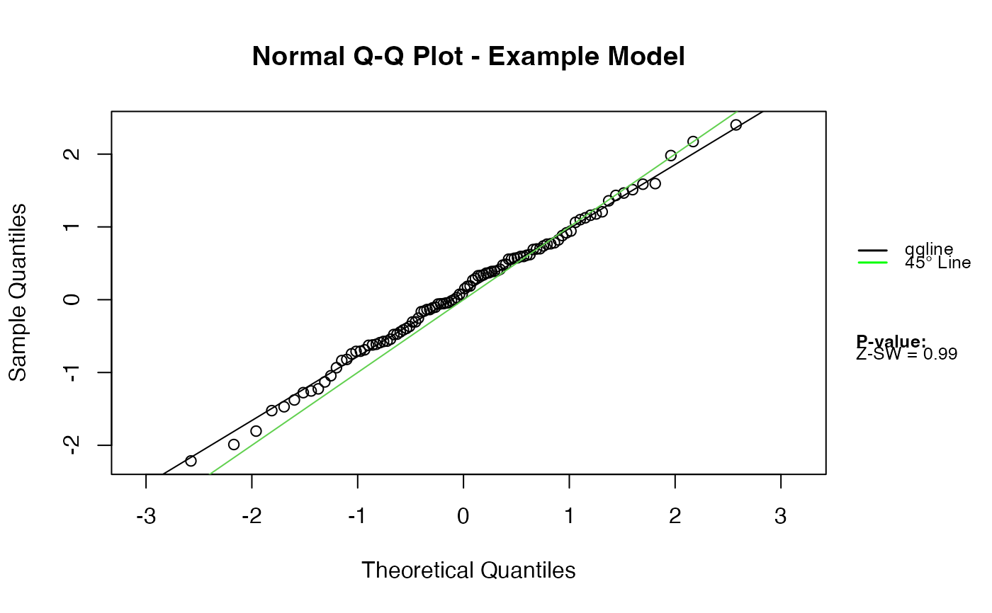
Produces a normal Q-Q plot for Z-residuals, with optional Shapiro–Wilk normality testing, automatic handling of infinite and extreme values, axis breaks for very large residuals, and visual annotation of detected outliers. This diagnostic is designed for checking the normality assumption of Z-residuals obtained from Bayesian predictive model checks (posterior, LOOCV, ISCV, etc.).

Usage

# S3 method for class 'zresid'
qqnorm(
  y,
  irep = 1,
  diagnosis.test = "SW",
  main.title = ifelse(is.null(attr(y, "type")), "Normal Q-Q Plot",
    paste("Normal Q-Q Plot -", attr(y, "type"))),
  xlab = "Theoretical Quantiles",
  ylab = "Sample Quantiles",
  outlier.return = TRUE,
  outlier.value = 3.5,
  outlier.set = list(),
  my.mar = c(5, 4, 4, 6) + 0.1,
  legend.settings = list(),
  ...
)

Arguments

y: A numeric matrix of Z-residuals where each column corresponds to an iteration or predictive draw. The function also uses the attribute "type" (optional model name) to construct default titles.
irep: Integer or vector of integers indicating which column(s) of Zresidual to plot. Defaults to 1.
diagnosis.test: Character string indicating the normality test to perform. Currently only "SW" (Shapiro–Wilk test; using sw.test.zresid()) is supported.
main.title: Main title of the plot. If missing, it is automatically constructed using the "type" attribute of Zresidual.
xlab, ylab: Axis labels for the Q-Q plot.
outlier.return: Logical; if TRUE, the function prints and returns the indices of detected outliers.
outlier.value: Numeric threshold used to classify an observation as an outlier based on |Zresidual| > outlier.value. Default is 3.5.
outlier.set: Optional named list of graphical parameters passed to symbols and text for customizing the outlier annotation.
my.mar: Numeric vector giving margin sizes, passed internally to par(mar = ...). Default is c(5, 4, 4, 6) + 0.1.
legend.settings: Optional named list of parameters to override default legend appearance settings.
...: Additional graphical arguments passed to qqnorm and plot.

Value

Invisibly returns a list with:

outliers: An integer vector containing the indices of detected outliers.

If no outliers are detected, an empty integer vector is returned.

A Q-Q plot is produced as a side effect.

Details

This function extends the base R Q-Q plot to better handle typical behavior of Z-residuals in Bayesian predictive checking:

Infinite values (Inf/-Inf) are replaced with large finite values and trigger a warning.
Very large Z-residuals (|Z| > 6) are shown using axis breaks to avoid plot distortion.
Outliers (|Z| > outlier.value) are highlighted and labeled.
Column-wise Shapiro–Wilk tests assess normality.
Legends summarize model type, selected Q-Q lines, and diagnostic results.

This diagnostic is suitable for Z-residuals such as randomized quantile residuals, posterior predictive Z-residuals, LOOCV/ISCV Z-residuals, and residuals from hurdle or zero-inflated Bayesian models.

References

Dunn, P. K., & Smyth, G. K. (1996). Randomized quantile residuals. Journal of Computational and Graphical Statistics, 5(3), 236–244.

Gelman, A., Carlin, J. B., Stern, H. S., Dunson, D. B., Vehtari, A., & Rubin, D. B. (2013). Bayesian Data Analysis. CRC Press.

Examples

library(Zresidual)
set.seed(1)
Z <- matrix(rnorm(200), ncol = 2)
attr(Z, "type") <- "Example Model"

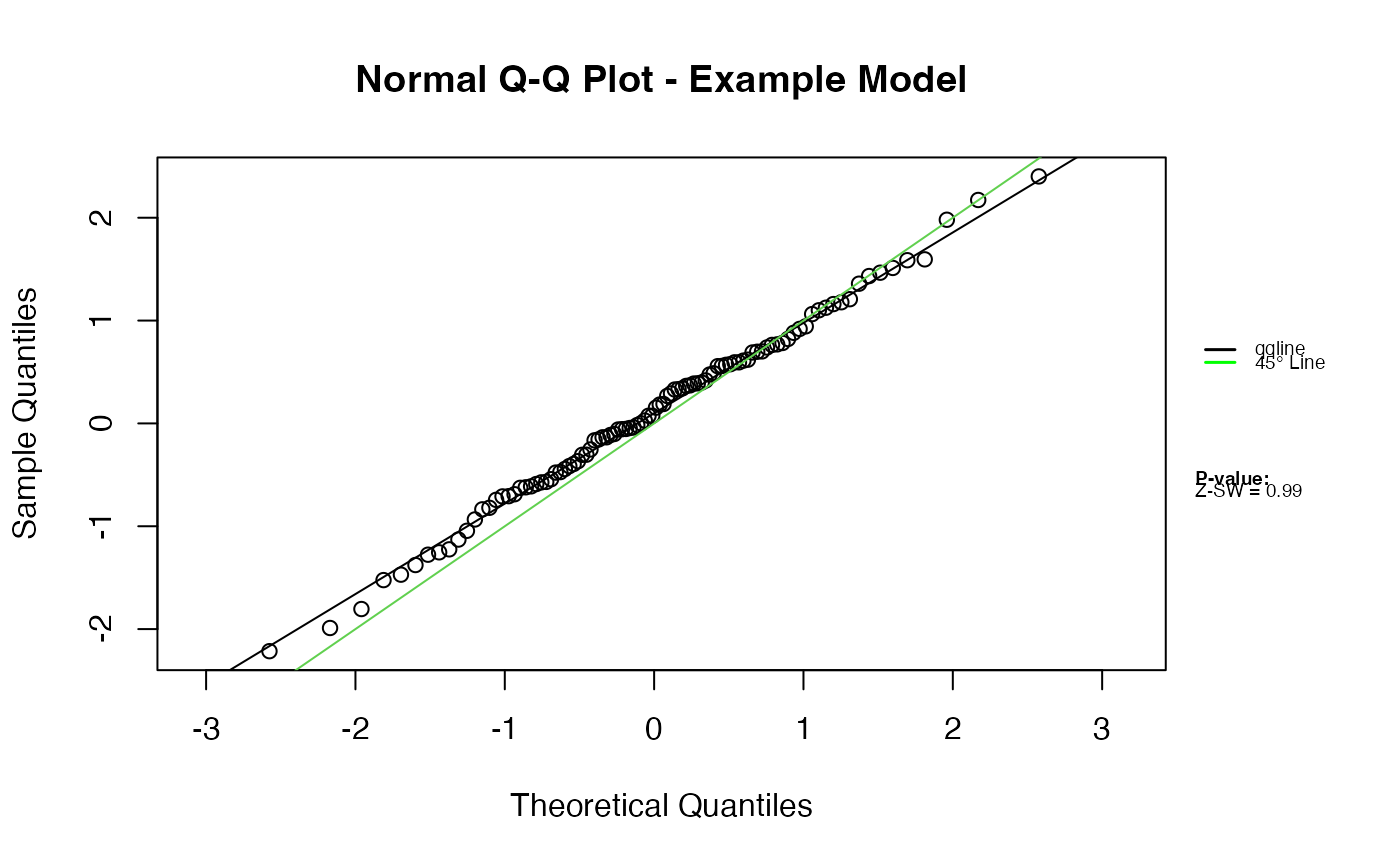
# Basic Q-Q plot
qqnorm.zresid(Z)


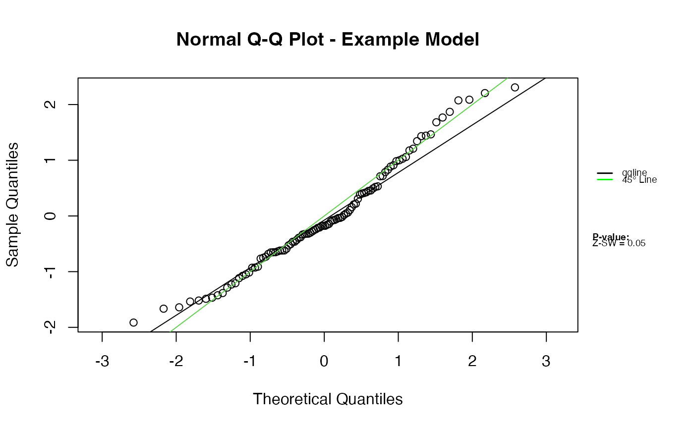
# Use the second column with custom outlier threshold
qqnorm.zresid(Z, irep = 2, outlier.value = 2.5)


# Modify legend settings
qqnorm.zresid(Z, legend.settings = list(cex = 0.8))