Code
# For developer use to refresh the local installation
remove.packages("Zresidual")
devtools::document()
devtools::install()2026-01-15
Source:vignettes/demo_coxph_survival.qmd
# For developer use to refresh the local installation
remove.packages("Zresidual")
devtools::document()
devtools::install()
if (!requireNamespace("Zresidual", quietly = TRUE)) {
  if (!requireNamespace("remotes", quietly = TRUE)) install.packages("remotes")
  remotes::install_github("tiw150/Zresidual", upgrade = "never", dependencies = TRUE)
}
pkgs <- c(
  "survival", "EnvStats", "foreach", "statip", "VGAM", "plotrix", "actuar",
  "stringr", "Rlab", "dplyr", "rlang", "tidyr",
  "matrixStats", "timeDate", "katex", "gt", "loo"
)

missing_pkgs <- pkgs[!vapply(pkgs, requireNamespace, logical(1), quietly = TRUE)]
if (length(missing_pkgs)) {
  message("Installing missing packages: ", paste(missing_pkgs, collapse = ", "))
  install.packages(missing_pkgs, dependencies = TRUE)
}

invisible(lapply(pkgs, function(p) {
  suppressPackageStartupMessages(library(p, character.only = TRUE))
}))

nc <- parallel::detectCores(logical = FALSE)
if (!is.na(nc) && nc > 1) options(mc.cores = nc - 1)This vignette explains how to use the Zresidual package to calculate Z-residuals based on the output of the coxph function from the survival package in R. It also demonstrates how Z-residuals can be used to assess the overall goodness of fit (GOF) and identify specific model misspecifications in semi-parametric shared frailty models. For a thorough understanding of the underlying theory, please refer to: “Z-residual diagnostics for detecting misspecification of the functional form of covariates for shared frailty models.”
We use Z-residuals to diagnose shared frailty models in a Cox proportional hazards setting where the baseline function is unspecified. For a group i with n_i individuals, let y_{ij} be a possibly right-censored observation and \delta_{ij} be the indicator for being uncensored. The normalized randomized survival probabilities (RSPs) are defined as:
S_{ij}^{R}(y_{ij}, \delta_{ij}, U_{ij}) = \left\{ \begin{array}{rl} S_{ij}(y_{ij}), & \text{if } \delta_{ij}=1, \\ U_{ij}\,S_{ij}(y_{ij}), & \text{if } \delta_{ij}=0, \end{array} \right. \tag{1}
where U_{ij} \sim \text{Uniform}(0, 1) and S_{ij}(\cdot) is the postulated survival function. RSPs are transformed into Z-residuals via the normal quantile function:
r_{ij}^{Z}(y_{ij}, \delta_{ij}, U_{ij})=-\Phi^{-1} (S_{ij}^R(y_{ij}, \delta_{ij}, U_{ij})) \tag{2}
Under the true model, Z-residuals are normally distributed. This transformation allows researchers to leverage traditional normal-regression diagnostic tools for censored data. Furthermore, normal transformation highlights extreme RSPs that may indicate model misspecification but could otherwise be overlooked.
We utilize data from 411 acute myeloid leukemia patients recorded at the M. D. Anderson Cancer Center (1980–1996). The dataset focuses on patients under 60 from 24 districts. Key variables include survival time, age, sex, white blood cell count (WBC), and the Townsend deprivation score (TPI).
We compare two models: the wbc model (using raw WBC) and the lwbc model (using log-transformed WBC).
Once the model is fitted, we calculate Z-residuals for both models using 1,000 repetitions to account for randomization in censored cases.
Under a correctly specified shared frailty model, Z-residuals should be approximately standard normal, so a Q–Q plot should closely follow the 45° reference line. Because Z-residuals are generated from randomized survival probabilities for censored observations, the realized Z-residual set (and any normality-test p-value) can vary from one randomization replicate to another.
To assess overall goodness-of-fit (GOF), we primarily use Q–Q plots, and we report the replicate-specific Shapiro–Wilk (Z-SW) normality-test p-value as a compact numerical summary. The animation below shows the first 10 randomization replicates for both candidate models.
gif_qq_name <- "qqplot_anim.gif"
gif_qq_path <- file.path(extdata_path, gif_qq_name)

if (is_dev && (force_rerun || !file.exists(gif_qq_path))) {
  gifski::save_gif(
    expr = {
      for (i in 1:10) {
        par(mfrow = c(1, 2), mar = c(4, 4, 2, 2))
        qqnorm.zresid(Zresid.LeukSurv.wbc, irep = i)
        qqnorm.zresid(Zresid.LeukSurv.logwbc, irep = i)
      }
    },
    gif_file = gif_qq_path, width = 800, height = 400, res = 72, delay = 0.8
  )
}

local_qq <- get_local_asset(gif_qq_name, extdata_path, local_assets_dir)
if (!is.null(local_qq)) {
  knitr::include_graphics(local_qq)
} else {
  par(mfrow = c(1, 2))
  qqnorm.zresid(Zresid.LeukSurv.wbc, irep = 1)
  qqnorm.zresid(Zresid.LeukSurv.logwbc, irep = 1)
}
Across frames, both models show QQ patterns close to the diagonal with no obvious tail inflation. In this LeukSurv example, the overall GOF check alone does not distinguish the two competing functional forms (raw WBC vs log-WBC); the more targeted covariate-specific diagnostics in Sections 4.5–4.6 are needed.
A key Z-residual diagnostic for model adequacy is homogeneity: after sorting observations by the linear predictor (LP) and splitting into (k) groups, the grouped Z-residuals should have (approximately) the same mean and variance across LP groups if the model is adequate. Graphically, we expect: - the LOWESS smooth in the Z-residual scatterplot vs LP to stay close to the horizontal line at 0, and - the grouped boxplots to show similar centers and spreads.
We report two replicate-specific p-values to summarize the LP-group homogeneity checks. Z-AOV-LP is the ANOVA F-test p-value for equality of the group means, and Z-BL-LP is the Bartlett’s test p-value for equality of the group variances. In the LeukSurv example, across randomization replicates both the WBC and log-WBC models typically produce relatively large Z-AOV-LP and Z-BL-LP p-values, consistent with the visual impression that the LOWESS smooth stays near 0 and the grouped boxplots have comparable centers and spreads. Overall, LP-based grouping does not provide strong evidence of lack of fit for either model in this dataset.
gif_lp_name <- "lp_anim.gif"
gif_lp_path <- file.path(extdata_path, gif_lp_name)

if (is_dev && (force_rerun || !file.exists(gif_lp_path))) {
  gifski::save_gif(
    expr = {
      for (i in 1:10) {
        par(mfrow = c(2, 2))
        plot(Zresid.LeukSurv.wbc, x_axis_var="lp", main.title = "Scatter: WBC Model",
             irep=i,add_lowess = TRUE)
        plot(Zresid.LeukSurv.logwbc, x_axis_var="lp", main.title = "Scatter: log-WBC Model",
             irep=i,add_lowess = TRUE)
        boxplot(Zresid.LeukSurv.wbc, x_axis_var = "lp", main.title = "Boxplot: WBC Model", irep=i)
        boxplot(Zresid.LeukSurv.logwbc, x_axis_var = "lp", main.title = "Boxplot: log-WBC Model", irep=i)
      }
    },
    gif_file = gif_lp_path, width = 900, height = 900, res = 96, delay = 1
  )
}

local_lp <- get_local_asset(gif_lp_name, extdata_path, local_assets_dir)
if (!is.null(local_lp)) knitr::include_graphics(local_lp)
In this dataset, the LP-based homogeneity diagnostic does not clearly separate the two candidate models. We therefore proceed to covariate-specific diagnostics to assess whether the functional form of the WBC effect is misspecified.
To diagnose functional-form misspecification for a specific covariate, we inspect Z-residuals against that covariate (or its transformed version) and test whether grouped residual means differ across covariate intervals. If the functional form is adequate, the LOWESS curve should remain near 0 and grouped boxplots should have similar centers.
Here we directly compare the WBC model plotted against wbc, and the log-WBC (lwbc) model plotted against logwbc.
In the LeukSurv data, when diagnosing the functional form against log(wbc), the log-WBC model typically shows a pronounced systematic (non-linear) pattern in the LOWESS smooth and clear differences in grouped means, leading to consistently small Z-AOV-log(wbc) p-values across randomization replicates (e.g., < 0.01 in the real-data analysis). By contrast, the WBC model does not show comparably strong evidence of misspecification in this view: its replicated Z-AOV p-values are generally much larger, in line with a flatter smooth around zero and more homogeneous grouped boxplots. This contrast remains stable across many randomization replicates (see Sections 5.2–5.3).
gif_wbc_name <- "wbc_anim.gif"
gif_wbc_path <- file.path(extdata_path, gif_wbc_name)

if (is_dev && (force_rerun || !file.exists(gif_wbc_path))) {
  gifski::save_gif(
    expr = {
      for (i in 1:10) {
        par(mfrow = c(2, 2), mar = c(4, 4, 1.5, 2))
        plot(Zresid.LeukSurv.wbc, x_axis_var = "wbc", main.title = "Scatter: WBC Model",
        irep=i,add_lowess = TRUE)
        plot(Zresid.LeukSurv.logwbc, x_axis_var = "logwbc", main.title = "Scatter: log-WBC Model",          irep=i,add_lowess = TRUE)
        boxplot(Zresid.LeukSurv.wbc, x_axis_var = "wbc", main.title = "Boxplot: WBC Model", irep=i)
        boxplot(Zresid.LeukSurv.logwbc, x_axis_var = "logwbc", main.title = "Boxplot: log-WBC Model", irep=i)
      }
    },
    gif_file = gif_wbc_path, width = 900, height = 900, res = 96, delay = 1
  )
}

local_wbc <- get_local_asset(gif_wbc_name, extdata_path, local_assets_dir)
if (!is.null(local_wbc)) knitr::include_graphics(local_wbc)
To quantify the homogeneity of grouped Z-residuals, we test whether the grouped residuals are “homogeneously distributed” by examining equality of group means using an ANOVA F-test (Z-AOV). In addition, we report Z-BL p-values from Bartlett’s test as a complementary check for equality of variances across the same groups.
Table 1 summarizes the first 10 randomization repetitions. In these repetitions, the LP-grouping diagnostics (Z-AOV-LP and Z-BL-LP) yield predominantly non-small p-values for both models, consistent with no strong evidence of non-homogeneity against the linear predictor. In contrast, the covariate-grouping test for the log-WBC specification (aov.lwbc) is consistently near zero, indicating strong group-mean differences across log(wbc) intervals.
| Summary of Residual Homogeneity Tests | |||||||
|---|---|---|---|---|---|---|---|
| aov.wbc.lp | aov.lwbc.lp | bl.wbc.lp | bl.lwbc.lp | aov.wbc | aov.lwbc | bl.wbc | bl.lwbc |
| 0.8701 | 0.7299 | 0.5704 | 0.0612 | 0.5868 | 0.0001 | 0.9885 | 0.2790 |
| 0.8412 | 0.9480 | 0.6401 | 0.1581 | 0.6530 | 0.0000 | 0.9172 | 0.2637 |
| 0.9724 | 0.7668 | 0.6459 | 0.7844 | 0.5199 | 0.0000 | 0.7273 | 0.5765 |
| 0.7362 | 0.8222 | 0.3540 | 0.8142 | 0.6979 | 0.0000 | 0.5464 | 0.6532 |
| 0.9054 | 0.6409 | 0.8773 | 0.2562 | 0.6199 | 0.0000 | 0.9712 | 0.1497 |
| 0.9276 | 0.7744 | 0.9451 | 0.7756 | 0.8013 | 0.0000 | 0.2140 | 0.5403 |
| 0.9730 | 0.8900 | 0.1287 | 0.1508 | 0.5196 | 0.0001 | 0.4639 | 0.9744 |
| 0.9149 | 0.8252 | 0.9055 | 0.3982 | 0.5772 | 0.0001 | 0.9324 | 0.6336 |
| 0.8917 | 0.5897 | 0.8742 | 0.1209 | 0.5520 | 0.0000 | 0.7991 | 0.9185 |
| 0.9076 | 0.6479 | 0.7593 | 0.2998 | 0.6597 | 0.0000 | 0.9469 | 0.7640 |
To connect the above visuals to the replicated-test summary used in the paper, the following compact table reproduces the LeukSurv comparison (AIC, CZ-CSF p-value, and p_{min} summaries over 1000 replicates). Notably, the log-WBC model fails the Z-AOV-log(wbc) diagnostic decisively, even though some overall-fit diagnostics (e.g., CZ-CSF and normality-based tests) do not flag this inadequacy.
| Model | AIC | CZ-CSF (p-value) | Z-SW (p_min) | Z-SF (p_min) | Z-AOV-LP (p_min) | Z-AOV-log(wbc) (p_min) |
|---|---|---|---|---|---|---|
| WBC model | 3,111.669 | 0.255 | 0.495 | 0.693 | 0.703 | 0.074 |
| log-WBC model | 3,132.105 | 0.305 | 0.579 | 0.781 | 0.978 | <1e-5 |
| $p_{min}$ is a conservative upper-bound summary for replicated p-values; a practical failure cutoff can be much larger than 0.05 (e.g., 0.25). | ||||||
These histograms reveal that the Z-SW, Z-SF, and Z-AOV-LP tests for both models have a substantial proportion of p-values greater than 0.05, leading to large pmin values. In contrast, the replicated Z-AOV-log(wbc) p-values for the lwbc model are nearly all smaller than 0.001, providing strong evidence that the log transformation of wbc is inappropriate for modelling the survival time.
pmin.sw.wbc<-pvalue.min(pv=sw.wbc); pmin.sw.lwbc<-pvalue.min(pv=sw.lwbc)
pmin.sf.wbc<-pvalue.min(pv=sf.wbc); pmin.sf.lwbc<-pvalue.min(pv=sf.lwbc)
pmin.aov.lp.wbc<-pvalue.min(pv=aov.wbc.lp); pmin.aov.lp.lwbc<-pvalue.min(pv=aov.lwbc.lp)
pmin.aov.wbc<-pvalue.min(pv=aov.wbc); pmin.aov.lwbc<-pvalue.min(pv=aov.lwbc)

par(mfrow = c(4, 2), mar = c(4, 4, 2, 2))
hist(sw.wbc, main = "Z-SW: WBC Model", breaks = 20); abline(v = pmin.sw.wbc, col = "red")
hist(sw.lwbc, main = "Z-SW: log-WBC Model", breaks = 20); abline(v = pmin.sw.lwbc, col = "red")
hist(sf.wbc, main = "Z-SF: WBC Model", breaks = 20); abline(v = pmin.sf.wbc, col = "red")
hist(sf.lwbc, main = "Z-SF: log-WBC Model", breaks = 20); abline(v = pmin.sf.lwbc, col = "red")
hist(aov.wbc.lp, main = "Z-AOV (LP): WBC Model", breaks = 20); abline(v = pmin.aov.lp.wbc, col = "red")
hist(aov.lwbc.lp, main = "Z-AOV (LP): log-WBC Model", breaks = 20); abline(v = pmin.aov.lp.lwbc, col = "red")
hist(aov.wbc, main = "Z-AOV (WBC): WBC Model", breaks = 20); abline(v = pmin.aov.wbc, col = "red")
hist(aov.lwbc, main = "Z-AOV (log-WBC): log-WBC Model", breaks = 20); abline(v = pmin.aov.lwbc, col = "red")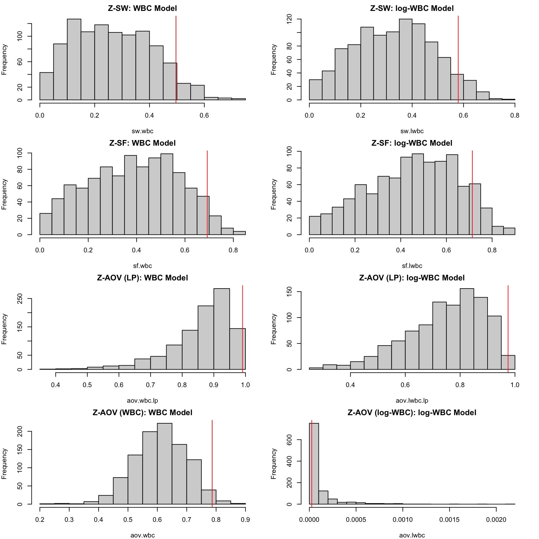
We first report the CZ-CSF p-values, where “censored Z-residuals” are defined by r^{n}_{ij}(t_{ij}) = -\Phi^{-1}\!\left(\widehat{S}_{ij}(t_{ij})\right), and normality is assessed using the SF test for multiply censored data (EnvStats::gofTestCensored).
As an overall goodness-of-fit check, CZ-CSF evaluates the residual distribution but does not assess specific model assumptions such as the functional form of covariates.
| Model | CZ-CSF p-value |
|---|---|
| wbc model | 0.5702 |
| lwbc model | 0.0754 |
The Cox–Snell residual is defined as r^{CS}_{ij}(t_{ij}) = -\log\!\left(\widehat{S}_{ij}(t_{ij})\right).
Overall GOF checks based on CS residuals are commonly used, but they may not provide sufficient information about specific model inadequacies (e.g., the functional form of a covariate).
ucs.wbc <- surv_residuals(fit.object = fit_LeukSurv_wbc, data= LeukSurv, residual.type = "Cox-Snell" )
ucs.lwbc <- surv_residuals(fit.object = fit_LeukSurv_logwbc, data= LeukSurv, residual.type = "Cox-Snell" )
par(mfrow = c(1, 2)); plot.cs.residual(ucs.wbc, main.title = "CS Residuals: WBC Model"); plot.cs.residual(ucs.lwbc, main.title = "CS Residuals: log-WBC Model")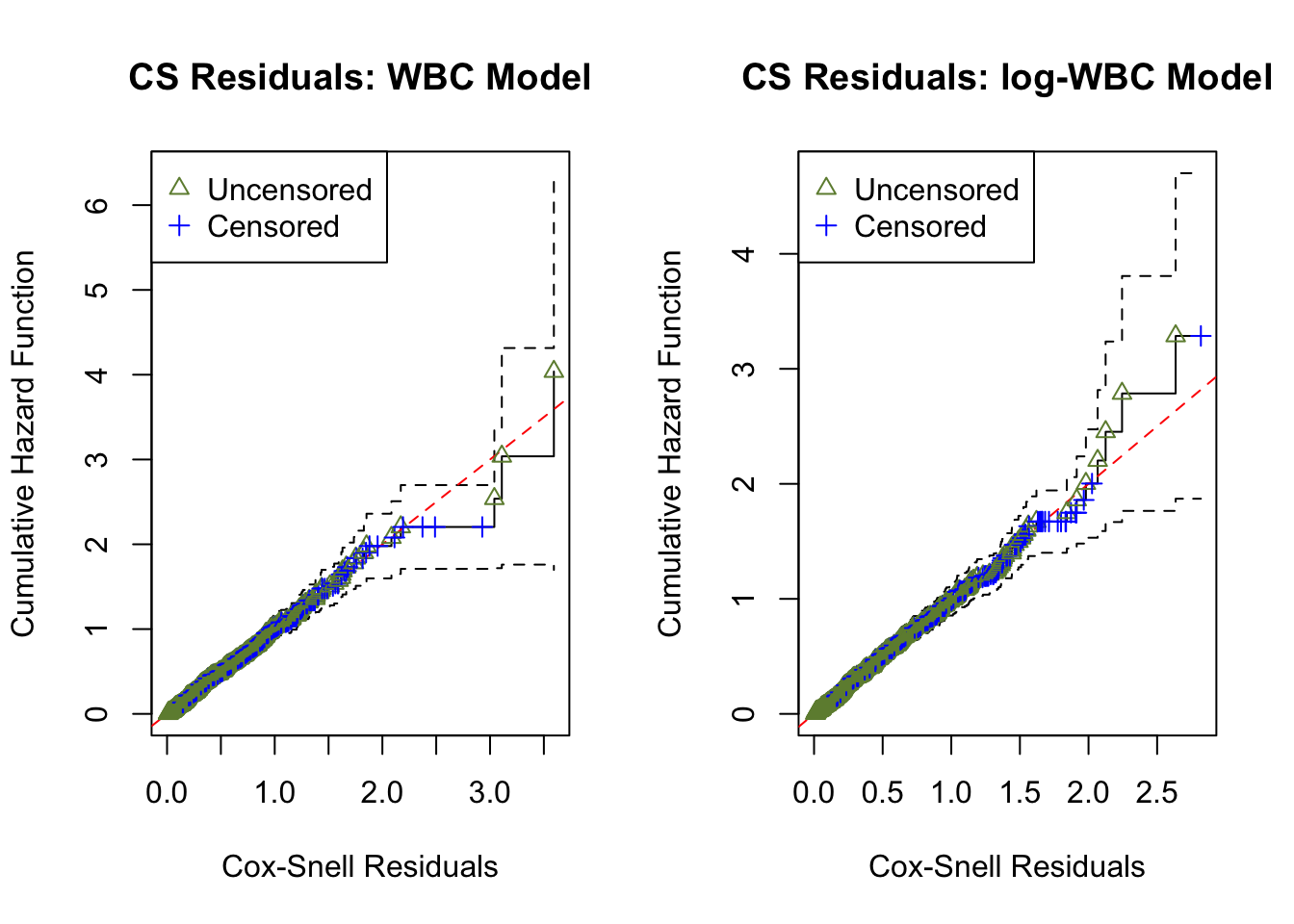
To gain further insights, residual scatterplots are often augmented with LOWESS lines; however, the visual interpretation can still be subjective, and numerical tests are difficult to derive because these residuals lack a reference distribution under censoring.
martg.wbc <- surv_residuals(fit.object = fit_LeukSurv_wbc, data= LeukSurv, residual.type = "martingale")
martg.lwbc <- surv_residuals(fit.object = fit_LeukSurv_logwbc, data= LeukSurv, residual.type = "martingale")
par(mfrow = c(1, 2))
plot.martg.resid(martg.wbc, x_axis_var="wbc", main.title = "Martingale Residuals: WBC Model")
plot.martg.resid(martg.lwbc, x_axis_var="logwbc", main.title = "Martingale Residuals: log-WBC Model")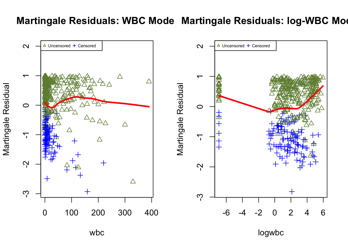
Although deviance residuals reduce skewness relative to martingale residuals and can improve visual assessment, objective numerical measures remain hard to construct under censoring because these residuals do not admit a convenient reference distribution.
dev.wbc <- surv_residuals(fit.object = fit_LeukSurv_wbc, data= LeukSurv, residual.type = "deviance")
dev.lwbc <- surv_residuals(fit.object = fit_LeukSurv_logwbc, data= LeukSurv, residual.type = "deviance")
par(mfrow = c(1, 2))
plot.dev.resid(dev.wbc, x_axis_var="wbc", main.title = "Deviance Residuals: WBC Model")
plot.dev.resid(dev.lwbc, x_axis_var="logwbc", main.title = "Deviance Residuals: log-WBC Model")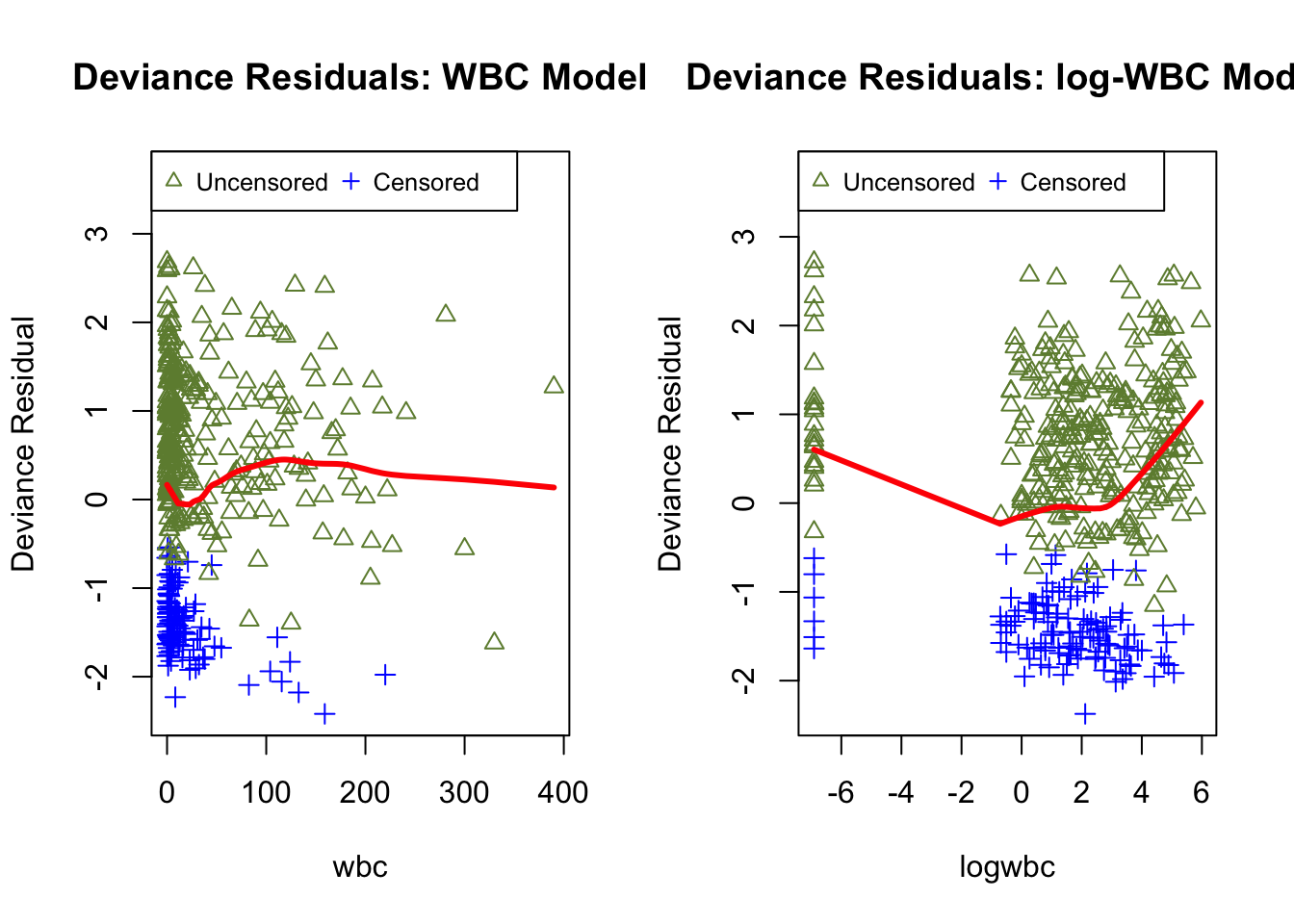
Wu, T., Li, L., & Feng, C. (2024). Z-residual diagnostic tool for assessing covariate functional form in shared frailty models. Journal of Applied Statistics, 52(1), 28–58. https://doi.org/10.1080/02664763.2024.2355551