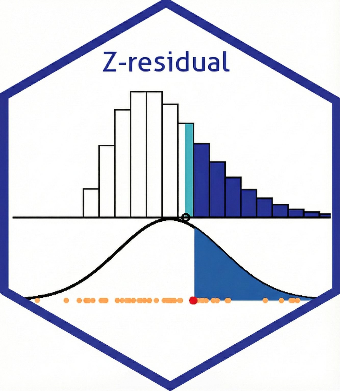
Z-residuals
The Zresidual package implements diagnostic residuals based on the predictive distribution of each observation. By utilizing the full probabilistic information of the model, the package generates residuals that are approximately normally distributed. This allows for standard diagnostic techniques similar to using Pearson residuals in OLS regression.
RSP
For a given observation y_i, the Randomized Survival Probability (RSP)—also known as the randomized probability integral transform—represents the value of the predictive survival function (upper-tail probability) at y_i, adjusted with a randomization term to ensure continuity for discrete outcomes. It is defined as:
RSP_i(y_i \mid \theta) = S_i(y_i \mid \theta) + U_i \, p_i(y_i \mid \theta) \tag{1}
where S_i and p_i represent the survival function and probability mass function, respectively, derived from the predictive distribution of y_i given covariates \mathbf{x}_i and parameters \theta. U_i \sim \text{Unif}(0,1) is a random uniform variable used to smooth discrete outcomes. Under a correctly specified model—where the observed data y_i arises from the assumed predictive distribution—the RSP follows a \text{Unif}(0,1) distribution.
Z-residual
The Z-residual (aka randomized quantile residual) is derived by transforming the RSP via the inverse survival function of N(0,1):
z_i(y_i \mid \theta) = -\Phi^{-1}\left(RSP_i(y_i \mid \theta)\right)= \Psi^{-1}\left(RSP_i(y_i \mid \theta)\right) \tag{2}
where \Psi^{-1}(p) = -\Phi^{-1}(p) = \Phi^{-1}(1-p) represents the inverse survival function (upper-tailed quantile) of the standard normal distribution N(0,1).
In words, the Z-residual is simply the N(0,1) value that shares the same upper-tail area (RSP) as the observed y_i. This transformation effectively maps any predictive distribution to the standard normal scale while preserving the tail probabilities. If the model is correct, the resulting Z-residuals follow a standard normal distribution.
Intuition:
Think of the Z-residual as the distance to the median, but rescaled to account for skewness and smoothed to handle discreteness. This ensures that a residual of +2 always implies the same degree of ‘extremeness’, regardless of the original distribution’s shape.
Z-residuals of a True Model
The animation in Figure 1 demonstrates this transformation for y_i using its true predictive distribution. As more points are simulated, the distribution of z_i values (shown by the accumulating points) aligns with the theoretical N(0,1) density curve.
Z-residuals of a Wrong Model
The animation in Figure 2 demonstrates the behavior of Z-residuals when the model is misspecified. Here, the data y_i are simulated from a True Model (Negative Binomial with \mu=2), but the residuals are calculated based on a Postulated Model (Negative Binomial with \mu=5).
We can see that the observed data (solid bars) fall systematically to the left of the expected distribution (dashed bars). Because the observed values are smaller than expected, the calculated RSP values are consistently high (upper tail area is large), resulting in z_i values that drift toward the negative side of the standard normal distribution.
